Quantcast
Channel: The RAS Solution
Viewing all 200 articles
Browse latest View live

Lifting Terrain in HEC-RAS 5.0

$
0
0
Written by Gerrit Kiers |  VIZITERV Consult Kft., Hungary
Copyright © The RAS Solution and Gerrit Kiers 2015.  All rights reserved.

Using Cross Section Data to add a levee


It is a common problem in hydraulic modeling that terrain data does not include the actual terrain underneath the water surface. With HEC-RAS 5.0 a terrain model can be improved by adding channel bathymetry to the existing terrain surface with the Cross Section Data (see Chapter 2 of the 2D Modeling User's Manual, or visit http://hecrasmodel.blogspot.com/2014/12/including-channel-bathymetry-into-your.html).

With this procedure it is also possible to locally lift the terrain, for instance on locations where a new levee alignment is planned. I use the Cross Section Editor to define a levee as an inverse channel that will be standing out above the existing surface. Then I create a levee terrain model and add that levee model to the existing terrain surface.

For the following example, I used the Muncie 2D HEC-RAS dataset that comes with HEC-RAS 5.0.0 Beta March 2015. One of its geometries contains break lines in the 2D Flow Grid. It is important to define break lines along the levees to make sure that flow across the cell faces is blocked by the elevation of the levee along the break line. In this example it is fortunate that these break lines were already defined so I was able to use their alignment for my levee.

000

For the definition of the levee I created a new geometry file and in this geometry I drew a river reach (Muncie levee) just on top of the break lines.

001

Constructing the cross section data for the new levee is rather straightforward. In this example I created the levee on a fixed elevation of 950 ft. There is no need to extend the side-slopes so that they touch the actual surface, but they do have to be pointing downwards. I added two identical cross sections on both ends of the levee.

002

There are two additional aspects to be aware of at this phase. First of all, make sure that the levee is wide enough to be represented in the terrain model you create. That is strongly related to the cell size of the terrain model. In this example a levee of 20 ft width will be more than sufficient as the Muncie terrain has a cell size of 5 ft x 5 ft Secondly, one also needs to check if the levee is consistently defined above the existing surface level, since we don’t want the levee to cut into existing terrain. If the alignment runs into natural high ground, one can locally lift the levee above the terrain level by adding extra cross sections. It is also possible to split the levee into separate reaches, before and after the high ground section.

With the current Beta version it is important to generate multiple cross sections by interpolation before creating the levee model. I opted for interpolation at every 100 ft.

007

At this point I was able to export the levee model as a terrain model. For this I used the ‘Create Terrain GeoTIFF from XS's’ option, accessible from the data file tree on the left in RAS Mapper. Right-click on the name of the geometry file you’re working in and select Export Layer… Create terrain GeoTiff from XS’s. In my example the ‘Channel Only’ option is sufficient. I named my terrain LeveeOnly.

008

There is only one step left, the joining of the original terrain model with the ChannelOnly terrain and the LeveeOnly terrain to create a terrain model that includes all features we want represented in the terrain. From RAS Mapper I invoked the menu option "New terrain" and added the different terrain models to the listing, as can be seen in the next screen capture. As the channel and levee must have higher priority for this procedure, they were moved to the top of the list.

010

The new terrain 'TerrainWithChannelAndLevee' includes both the channel bathymetry and the aligned levee.

016

On closer inspection we can see that there is an issue with the levee in one of its bends. Due to the cross section spacing of 100 ft, the LeveeOnly terrain appears cut off.  Tighter cross section spacing will improve this.  Notice that there is also an issue with the grid cells at this location. There is one 2D cell whose face does not match the break line alignment. Closer cell center spacing assigned to that break line should improve this situation.

017

Consequently, this bend will allow for some leaking along the different cell faces. In a real world situation I would need to address both issues before I can continue with my calculations. For now I neglect these and want to see how my new terrain performs.
For that purpose we can calculate one of the defined examples with the new terrain model. In the next screenshot we see the flooding caused by the upstream river levee breach with the original terrain, as modeled in the plan ‘Unsteady Run with 2D 50ft User n Value R’.

019

In the next screenshot we see the same flood event with the new terrain. It is clearly visible how the new levee performs in protecting lower areas, even though some leakage is visible. This leakage is due to the abovementioned issues in the terrain at the levee bend. This leakage can be eliminated by more refinement of the levee in the terrain (i.e. closer cross section spacing) and by better alignment of the adjacent cells using breaklines with smaller cell center spacing.

020

With this I hope to have demonstrated that the use of the Cross Section Data in HEC-RAS 5.0 is a very efficient tool for defining levee alignments in HEC-RAS 5.0. This new concept is relatively easy and can be used to define multiple terrain models with different levee alignments, which can be used in the evaluation of different flood protection scenarios.

Disclaimer: These model runs are only generated as examples to demonstrate the new abilities of HEC-RAS 5.0.0 Beta.

Gerrit Kiers is a Dutch hydrologist, working for VIZITERV Consult Kft. in Hungary.  Thank you Mr. Kiers for sharing your idea for terrain lifting in HEC-RAS 5.0!

Mr. Kiers' data set that demonstrates this technique can be downloaded here:  https://drive.google.com/file/d/0B0bpiyLiUeRXbC1rTmF4bUJvQjQ/view?usp=sharing


Windows 8 Compatibility Issues

$
0
0
If you are a Windows 8 user and you are having trouble getting HEC-RAS Version 5.0 beta to work, Window's Program Compatibility Troubleshooter may solve the problem.  Problems usually arise when pressing the compute button.  One common message that pops up is "Error starting process.
Steady file not found." The Program Compatibility Troubleshooter will fix this.

In Windows 8, you can get to the Program Compatibility Troubleshooter and learn how to use it for HEC-RAS by following the instructions here:
 http://windows.microsoft.com/en-us/windows-8/older-programs-compatible-version-windows

Using User-Defined Curves for Gates

$
0
0

Written by Christopher Goodell, P.E., D.WRE  |  WEST Consultants
Copyright © The RAS Solution 2015.  All rights reserved.

HEC-RAS allows for four different gate types that will compute the stage-discharge relationship of that gate for you based on the physical size/shape of the gate and a few empirical coefficients:  Sluice Gates, Radial Gates, Overflow Gates (closed top) and Overflow Gates (open air).  However, sometimes the built-in gate types don’t quite fit the gate that you want to simulate.  Or perhaps you have a unique spillway that can’t be captured adequately with the simple weir equation that HEC-RAS uses.  Either way, if you can come up with your own rating curve (state-discharge relationship) for the gate or hydraulic structure, you can model it accurately in HEC-RAS using the “User Defined Curves” gate type. 

image

As you can see, the User Defined Curves, although not a gate “type” in the literal sense, is added as the fifth gate type that you can choose from.  To use User Defined Curves, first add a new gate group to your inline structure (can also be used with lateral structures or SA/2D area connections) by entering in some geometric properties.  When using curves, the height and width are inconsequential-they don’t matter, because they won’t be used.  Just make sure that the height is at least as high as the highest gate opening setting you will use.  The invert is important, because that is what determines at what stage HEC-RAS will begin using the rating curves.  The centerline stationing just tells HEC-RAS how many gates you will have.  Again, the actual  stationing is inconsequential, just make sure you have the correct number of stations included.  Finally, enter in the user defined curves by pressing the Enter/Edit User Defined Curves… button. 

image

After entering the User Defined Gate Performance Curves window for the first time, you’ll notice that you must click on the “New” button image  to start a new set of curves.  Click New, then enter a name for the curves set. 

image

The first column, column 1, starting below the Gate Open Ht\HW entry, put in gate openings you wish to define curves for.  Each gate opening will have its own rating curve.  If you are putting in just a single rating curve (e.g. a spillway-maybe a morning glory type spillway), I always put in a zero gate opening curve in row 2 (with values of zero discharge for each headwater entry) and then the gate opening I wish to define goes in row 3.  No need for any more rows to be entered for single rating curves  The “zero” curve may or may not be necessary.  It seems to change with each new version of HEC-RAS.  Also, with a single rating curve, the gate opening value you enter in the first column really doesn’t matter.  It can be anything as long as it is equal to or less than the arbitrary gate height you defined in the gate editor AND it is the gate opening you use for the unsteady flow editor boundary condition (more on this in just a bit).  For a family of curves, you’ll want to put in a curve for a number of different gate openings, spanning the range of gate openings you plan to use in the simulation. 

Next enter in some headwater elevations (HW) in the first row.  You need at least 2 HW entries so that HEC-RAS can interpolate/extrapolate if necessary.  But the more HW values you enter, the more definition you’ll have.  The first headwater entry should be the invert of the gate (or spillway) and should get all zero values for discharge in that column.  The last headwater entry should be equal to or greater than the largest stage you expect to have in the forebay (although it doesn’t have to be, HEC-RAS will extrapolate). 

image

Press the Plot… button just to make sure that the curves look correct.

image

The final step is to go into the unsteady flow editor and set an internal boundary condition for the user defined gates.  You can select from Time Series Gate Openings (T.S. Gate Openings), Elevation Controlled Gates, Navigation Dams, or Rules).  Typically you’ll stick with one of the first two, the latter two are for advanced applications.  If you have a single rating curve, select T.S. Gate Openings and then just enter in the gate opening you have in the user defined curves for the entire simulation.  If you have a family of curves (as illustrated above), you can use T.S. Gate Openings or Elevation controlled gates, which ever suits your needs.  Elevation controlled gates allows HEC-RAS to determine how much to open the gate(s), based on the water surface elevation at a target location.  With T.S. Gate Openings, you simply tell HEC-RAS what the gate opening will be for each computation interval. 

image

Now you’re ready to compute.

2D Modeling with HEC-RAS Training in Italy!

$
0
0

Who wants to meet up in Milan, Italy for some 2D HEC-RAS training?!?!  I’ll be giving this course with help from Antonio Cotroneo on November 10-12, 2015.  The course will be given in English with Italian translation.

This intensive, three day course will prepare the engineer and water resource professional to use HEC-RAS 5.0 for modeling two-dimensional
(2D) flow. Led by Chris Goodell, P.E. D.WRE Manager, Director of Applied Research. WEST Consultants, Inc. Portland OR (USA), with the collaboration of Antonio Cotroneo, Italian Hydraulic Engineer. The participants will learn how to approach and construct a 2D model for unsteady flow conditions, and to effectively view and analyze results. HEC-RAS 5.0 incorporates various aspects of 2D hydraulic modeling, including combined 1D and 2D systems.

TrainingSacramento


Follow the link for more information and to enroll:  https://drive.google.com/file/d/0B0bpiyLiUeRXZmtiZWpEQ05KMW8/view?usp=sharing


Please direct questions to Antonio Cotroneo at cotroneo79@gmail.com

Hope to see you there!

  20150203_122235


Combining Two Reaches or Splitting One

$
0
0
Written by Christopher Goodell, P.E., D.WRE  |  WEST Consultants
Copyright © The RAS Solution 2015.  All rights reserved.

Suppose you have two separate HEC-RAS rivers and wish to combine them.  There is no “combine two rivers” option in HEC-RAS, but it can be done using the Move Points/Objects option.  Take the very simple reach presented below:

image

I wish to combine the Upper Tualatin with the Clackamas reach of the Willamette River.  In the figure above, they are disconnected-two separate rivers.  Select Edit…Move Points/Objects and
you’ll notice your cursor change to a pointer with an arrowed cross, and the vertices of the cross section and stream centerlines will highlight.


image

It’s helpful to zoom in close so you can see the end point nodes and so that you don’t accidentally grab a cross section node. 

image

Now simply grab the end point of one river and drag it on top of the end point of the other and release the mouse button. 

image

HEC-RAS will assume you want to put a junction here and will ask you what you want to name it.  It doesn’t matter what you put in for a name, because you will be deleting the junction next.

image

Make sure to uncheck the option to Move Points/Objects and then select Edit…Delete…Junctions.

image

Delete the temporary junction and you’re done.  You may need to close and reopen the HEC-RAS geometry schematic to make it look visually correct.

image

HEC-RAS will automatically take the name of the upstream of the two rivers for the new combined reach.  You can change the name of the river and/or reach using the Edit…Change Name menu item.  It is very important that your river stationing for the two reaches are consistent prior to doing this operation, or it will not work.  River stations must always be in descending order from upstream to downstream.
Now let’s say you want to do the reverse and split a single reach into two reaches.  This two involves a temporary junction.  But to get HEC-RAS to insert a junction, you must draw a temporary tributary river.  You can see in the figure below a new river has been drawn from the upper right to the point on the original river where I want to split it.  Double click the end of the line right on top of the existing river, so that HEC-RAS will recognize you want to create a junction. 

image

First HEC-RAS will ask you for the name of the new river/reach.  Again, the name doesn’t matter, we’ll be deleting it later. 

image

Next, HEC-RAS will ask if you wish to split the reach.  Say yes.

image

Now you have to give a new name for the reach below the split.  I’ll call it Willamette Clackamas, to take it back to the original two reaches I started with.

image

Now enter a temporary junction name.

image

If HEC-RAS asks if you want to increase the schematic extents, select Yes.  Now we have a river that was split into two by creating a temporary junction.

image

Since the temporary river and the temporary junction were only used to split the original river into two, go ahead and delete them using Edit…Delete…Junction and Edit…Delete…Reaches.
Now the rivers are disconnected, but they still don’t look like it in the schematic.  You can verify that they are disconnected by checking to see if the new river and reach name show up or by clicking on one and seeing how HEC-RAS highlights it.  Notice here only the lower of the two rivers is highlighted when I click on it.

image

If you want to visually make them look disconnected, use the Edit…Move Points Objects option again to pull the end points of the streams apart.  Again, it helps to zoom in to do this. 

image

Uncheck Edit…Move Points/Objects, and we’re done.  If you want it to look exactly like before, you can drag the stream centerline endpoints all the way back to the cross sections, but this is not necessary and has no effect on the computations. 

image

New Beta Version of HEC-RAS 5.0

$
0
0
Fellow HEC-RAS users:
A new beta version of HEC-RAS (August 21, 2015 build) is now available to download and install.  I have no new information about  when the final release will be made available, but for now this new beta version has a lot of bugs fixed and many new features, including breaklines, Manning’s n value regions, and mapping of sloped water surfaces in RAS Mapper for 2D areas.  Please follow the directions from HEC below for downloading and installing.
Enclosed is a link to a new HEC-RAS 5.0 version, Release Candidate 2, August 2015.  We have fixed several Bugs since the Release Candidate 1 version.  This version has all the features we have planned for the final release.  We are in a No New Features mode, and performing the final testing and documentation updates.
     Here is the link:
https://drive.google.com/file/d/0B0bpiyLiUeRXVEZyVWJVd0FNNUk/view?usp=sharing
     This self extracting exe should be run in a separate directory.  Once it is run, there will be a new Setup package for the HEC-RAS 5.0 beta software; a new 2D User’s Manual in PDF format; and a new set of 2D example data sets in a zip file.  You must have admin privileges to run and install the software using the setup package.  Please Uninstall the previous HEC-RAS 5.0 beta first!!!!
     Thank you for installing and testing this final Beta version of the software.
Some of the New Stuff:

1. Lateral Structures can now be Georeferenced.  So it will be easier to lay them out, and get them connected to 1D river reaches and 2D Flow Areas.
2. HEC-RAS Mapper, now uses a TIN based sloping water surface technique to show spatial results inside of RAS Mapper. Previous versions, in 2D area the depth, velocity, etc.. was plotted as a single value for the entire cell, which produced some blocky looking plots in steep terrain.
3. More flexible internal hydraulic structures.
4. Improvements to the stability of connecting 1D reaches into and out of 2D flow areas.
5. Several New output capabilities in RAS Mapper – please see the 2D user’s manual.
6. Many Bug fixes, especially in RAS Mapper.


Transect for Extracting Flow in a 2D Area

$
0
0

Written by Christopher Goodell, P.E., D.WRE  |  WEST Consultants
Copyright © The RAS Solution 2015.  All rights reserved.

A very common output request in 2D modeling is for flow over (through) a transect line.  HEC-RAS 5.0 does not have a specific tool for extracting flow data along a line in a 2D area, however it CAN be done.  Here’s how you do it.

Inside your 2D area, draw a 2D Area Connection where you would like to extract flow.  In the figure below, I’ve drawn my 2D Area Connection line from bottom to top, which represents left to right, looking in the downstream direction. 

image 

Notice that with the completely orthogonal cell orientation, but with a skewed 2D Area Connection line, the black and red striped connection line is “jagged”, following cell faces between the connecting cells.   To fix this, we need to use a breakline.  You could draw a break line on top of the 2D Area Connection (click the 2D Area Break Lines button on the top of the Geometric Data window), however, HEC-RAS also has a short cut for putting breaklines on 2D Area Connections.  If you right click on the 2D Area Connection (I’ve named if “Flow Line”), you’ll see an option to “Create 2D Flow Area Breakline”.  Select this for quick cell re-orientation around the 2D Area Connection Line.

image

image

Now you’re ready to enter data to the 2D Area Connection that you’ll use for extracting flow.  Click the SA/2D Area Conn button on the left side of the Geometric Data window. 

Make sure you connect “From” and “To” to the same 2D flow area.  Then choose “Normal 2D Equation Domain”.  This will force RAS to use the same 2D St. Venant equations over the terrain under the 2D Connection line as if the connection line wasn’t there.  BUT…you still have to define the Structure Type as a Weir and provide station-elevation data to define the crest of the weir, even though RAS will not use it.  Maybe this gets fixed in a later version.  HEC makes this easy though as you can extract the terrain profile from the 2D Connection cutline by clicking the button “Terrain Profile” as shown below.  Just copy and paste the terrain profile into your station-elevation table and you will  have defined a “zero-height” weir.  I guess it’s possible to use any crest definition, since RAS shouldn’t use the weir equation-it will use the normal 2D equation domain, but I haven’t tried it. 

image

Now you are ready to compute.  After computing, go to the Stage and Flow Hydrographs output window.

image

Make sure you select Type…Storage Area Connections (yes, it is technically an SA/2D Area Connection, but HEC hasn’t gotten around to renaming this yet in this window).  Now you can see the flow hydrograph for the flow line you’ve drawn.  You can check, but you’ll see the results are exactly the same as before including the flow line.


image

A Summary of New Features of the latest (Aug 21, 2015) beta version of HEC-RAS 5.0


Breaking the HEC-RAS Code – 1 Year!

$
0
0
Well it’s been one year since I published “Breaking the HEC-RAS Code”.  It was a lot of work, but I am very pleased to see how many people are making use of the book controlling and automating HEC-RAS with their own codes.


For those of you who haven’t discovered it yet, this book introduces the HECRASController, an API that gives you the ability to control HEC-RAS from an external application.  If you have HEC-RAS installed on your computer, you already have the HECRASController!  The book is written around Visual Basic for Applications (VBA), since most HEC-RAS users have Excel and many are already at least somewhat familiar with the VBA programming language embedded within.  However, many readers of my book have expanded the concepts presented to other programming codes like Python, R, C#, Matlab, etc with great success. 

“Breaking the HEC-RAS Code” unlocks the secrets to using the HECRASController.  If you would like more information about this book, or the companion Excel workbook that contains code written for every HECRASController procedure plus example code for a variety of applications, follow the link below or shoot me an email. 

Breaking the HEC-RAS Code

For those of you already making use of the HECRASController, let me suggest visiting The RAS Solution forum and posting examples and/or questions about your experience to the HECRAS Controller sub-forum.  Good luck breaking the HEC-RAS code!

Pressure and Weir Flow

$
0
0
Here’s a video of pressure and weir flow yesterday at a bridge near my house.  This was brought on by some very intense rainfall over a short period of time.  What do you think the weir coefficient would be?


‘Tis the season in many parts of the world for heavy rains and high water.  This is a good reminder to always try to get out and view your rivers and streams when they are flooding.  There is nothing like a first-hand view of a flood to understand how water interacts around our infrastructure.  This is invaluable information for setting up and calibrating your HEC-RAS models. 

HEC-RAS 5.0 versus TUFLOW versus MIKE21 – HEC’s official response

$
0
0
In case you haven’t seen it, there has been a very popular LinkedIn discussion on the Hydraulic/Hydrologic Modeler’s Forum debating the advantages, disadvantages, and merits of HEC-RAS 5.0, TUFLOW, and DHI’s MIKE21.  There was a lot of great information (and some misinformation) and insight provided in that thread.  It is well worth the read.  Some of the misinformation was directed at the beta version of HEC-RAS Version 5.0.  Enough that HEC decided to publish a response to clear up any confusion.  
At play is a result of HEC-RAS’s 2D solution scheme using the full shallow water equation where for highly dynamic events where flows severely contract, using too small of a time step could lead to a divergence from the true solution, rather than a convergence.  This is not an issue when a computation interval is selected within the guidance presented by HEC in their user’s manual.  While HEC disagrees that this is a necessarily a “problem” with its software, as some on the discussion claim,  HEC has elected to make this a non-issue by “improving the portion of the full shallow water equation formulation, such that user’s will be able to use very small time steps without the results changing significantly.”   I’ve included HEC’s response, written by Gary W. Brunner, to the LinkedIn discussion below, but I highly recommend you read the LinkedIn discussion first by clicking here
I’m posting this not just to allow HEC to reach a larger audience with their rebuttal, but also because there is a LOT of great information in this document about how HEC-RAS 2D works and how we, as HEC-RAS 2D modelers should use it.  Please enjoy!  A downloadable pdf is available here.
The following text is copyrighted by the Hydrologic Engineering Center and Gary W. Brunner:


This document is the official HEC response to the discussion on the LinkedIn forum:
Hydraulic/Hydrologic Modeler’s Forum
Discussion Tile:
Tuflow vs Mike DHI products vs HEC-RAS 5

Gary W. Brunner, HEC

            I am the lead Author/Developer of HEC-RAS.  In general, I do not respond to these types of discussions, because I feel it is wrong for software developers to comment about other software products, since they are generally not experts in software products, other than their own.  I also believe it is impossible for any software developer to be completely unbiased in such discussions, as we all think our individual products are the best and we know the most about our own software.  However, there has been so much speculation and misinformation stated about HEC-RAS in this discussion, I feel compelled to respond.

            I read through the discussion (several times), and will try to clear up any misconceptions, and what I consider to be misleading statements about HEC-RAS and its new 2D capabilities.

1.  HEC-RAS solves the full 2D shallow water equations, including Coriolis effects and representation of horizontal turbulent dispersion of momentum using an Eddy viscosity approach.   There was some discussion that some 2D models actually solve the 1D form of the Shallow water equations on a 2D mesh.  HEC-RAS does not do that. It solves the full 2D shallow water equations. 

2.  HEC-RAS uses a semi-Implicit, Eulerian-Lagrangian Finite Volume scheme.  Momentum advection is performed through a Lagrangian tracking step.  Friction, Coriolis, and hydrostatic pressure terms are solved implicitly with second order accuracy in space.  Eddy diffusion is formulated explicitly.  A modified Crank-Nicholson scheme is used in time, where the order of the scheme varies between linear and second order in time depending on the “theta” time weighting coefficient (1.0 is the default which is first order).   The solution scheme is described in full detail in the RAS technical documentation.  All of the details of how HEC-RAS works will be available in Chapter 2 of our technical reference manual, as always.  HEC always tries to be completely open about what equations we use, how we solve the equations, and what assumptions are made.  I believe this is very important in order for a user to truly understand how the software works (if they want to!).

3.  HEC-RAS has been applied to the European Environmental Agency (EA) 2D tests data sets by myself and others.  I have obtained excellent results on all of the data sets (1 -7), but was unable to run Test 8, as we do not currently have the capability to perform a combined 2D overland flow directly connected to a 1D underground pipe network yet. 

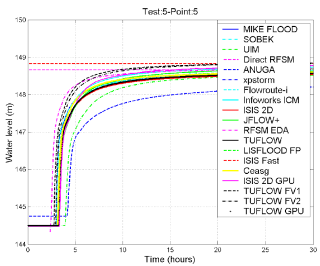
4.  There has been a lot of discussion and speculation about HEC-RAS and its sensitivity to the selection of the time step.  All of this discussion has centered around the results for a single test case, and only at a single location within that test case.  This is the Environmental Agency (EA) Test Case No. 5, and the results at only one location for test 5, (Point Location 5).   However, HEC-RAS is more than capable of producing exceptional results for this data set, at all locations (including test point 5), if the user picks a time step based on the guidance provided in the HEC-RAS 2D User's manual.

Here is a plot of HEC-RAS 2D results for Test Case 5, location 5, using multiple time steps of: 12, 10, 6, 5, 4, and 2 seconds:


Here is the plot from the 2013 Environmental Agency report (This plot was extracted from the Environmental agency report from 2013, entitled: “Benchmarking the latest generation of 2D hydraulic modeling packages”  Report – SC120002).  I think everyone involved in this discussion should download this report and review it closely.


            As you can see, the results from the original report have a very wide spread in the results from a range of 2D models.  Two of the models show straight lines, these are from simplistic 2D models that do not solve the full shallow water equations.  However, even for all the models that do solve the full shallow water equations, the results very widely.  If you compare the HEC-RAS results to the results shown at this location you will see that the HEC-RAS results for a wide range of time steps are well within the spread of all the other model results.  If you take away the HEC-RAS results for the 2 second time step run, all of the HEC-RAS results are very close together and fall right on top of the most widely used 2D models (TUFLOW, MIKE21, ISIS 2D, and SOBEK 2D).   All of the RAS results fall within the results shown in the study (even the ones run for the 2s time step).   For this test case (EA Test Case 5), the HEC-RAS results at all of the other locations are even tighter/much more consistent than this location.  Location 5 is the very most downstream location in which model results are being reported in this study, and is the one location where HEC-RAS shows significant variation in the results if you pick extremely small time steps. 

So, if a user follows the HEC-RAS guidance (for the full shallow water equation option) and picks a time step that will produce a Courant number around 1.0 for the high contraction and expansion zones in this data set (it can be lower or higher than 1.0), they will get very good results.   The HEC-RAS time step selection guidance is to find the locations within your model with the highest velocities, then to compute a time step that would produce a Courant number of around 1.0 for that location.

For this test case, the grid resolution specified by the test is 50 meters.  The highest velocities in the model occur at several very tight contractions in which the velocities go up to 5.0 to 6.0 m/s at different locations.  Based on these velocities, the best time step to be used for HEC-RAS would be around 10 seconds.  Why would anyone pick a time step that produces a Courant number of 0.1 or lower for the high velocity portion of the model?  In any practical application of the model they would not, as it would cause their model to run 10 times slower than necessary.  So, in general a user would not select a 1 or 2 second time step for this model if they were following the guidance in the HEC-RAS User’s Manual.

5.  Also shown in the HEC-RAS plot are two runs made with a 100 meter grid.  One with a 10s time step and one with a 15s time step.  As you can see, the results, even at Location 5, are very good.  The HEC-RAS model with the original grid (50 m grid) took 1 min 40s to run Test 5.  However, the 100 m grid with 15s time step only took 19 seconds.  This is one of the major benefits of what we are doing with the subgrid terrain.  The HEC-RAS 2D cells are pre-processed into detailed elevation-volume curves based on all of the information in the underlying terrain.  The elevation profile for each cell is extracted as a detailed cross section based on the underlying terrain.  Next, detailed elevation vs area, wetted perimeter, and roughness curves are developed for each face of each cell.  This allows HEC-RAS 2D to compute very accurate volumes based on the full sub grid terrain.  Because the cell faces are detailed cross sections, HEC-RAS has a very accurate estimate of the terrain under each cell face.  None of the other models mentioned in this LinkedIn discussion do that (to my knowledge at least.  If I am incorrect I apologize to whatever software may have this capability).  The other software packages reduce the elevation data within each computational cell down to a single elevation for each cell and each face is also a single elevation flat line.  Those software packages that use triangles, reduce the terrain down to three elevations (One elevation at the end of each side of the triangle) and each Face is a straight line with two elevations.  This is a huge difference compared to what we are doing in HEC-RAS 2D.

What HEC-RAS does by preprocessing the cells and faces into detailed curves based on the underlying terrain allows the user to use larger cells and still retain the detail of the underlying terrain.  Larger cells means fewer cells, which means faster run times.  As I pointed out above, HEC-RAS was able to run the EA Test Case 5 with a 100 meter grid and get basically the same results as using the 50 meter grid.  But it was able to do this at a speed that was more than 5 times faster.   This is a major feature of HEC-RAS that user need to take advantage of in order to get the most efficiency out of the HEC-RAS software.

6.  Given that the other models discussed in this forum reduce each cell to a single elevation (RiverFlow 2D uses triangles), and each cell face to a single straight line, this in itself could be producing bad results.  How accurate is the estimation of the channel shape, wetted perimeter, and volume underneath the computed water surface if you are only using 5 or so cells across the main channel, with models that reduce each cell to a single elevation.  This could produce a bad estimate for wetted perimeter, cross section shape and volume of the channel/floodplain, and will definitely affect the results the model produces.  Additionally, with these types of models, if you change the cell size, you will get different estimates for the channel shape, wetted perimeter, and volume within the channel and floodplain.  How does one pick a consistent Manning’s n value, if the wetted perimeter and channel shape and volume change when you change the grid resolution?  This means that roughness coefficients picked for these models are tied to the grid resolution, and they will need to be changed when changing grid resolutions.  But no one seems to be talking about the significance of this issue.  HEC-RAS allows the grid resolution to change and still maintain accurate estimates of the channel and floodplain shape, wetted perimeter, and volume underneath the water surface.  This reduces the necessity to have different Manning’s roughness values for different grid resolutions.

Assuming the user understands this issue about these models, and why it is true, they would need to first get a good grid resolution before performing any final calibration of the model.  In areas where there is no data to calibrate, it will require that the user has significant experience in using these models, under conditions where they did have observed data, to gain experience in picking roughness coefficients for those types of models.   Experienced modelers will know and understand this issue, but many user’s do not know or understand this. 

7.  HEC-RAS allows the user to pick time steps that are higher than a Courant number of 1.0.  So our solution has a wide range of possible time steps that will work and produce consistent and good results.  Some of the other models cannot have a time step with a Courant Number higher than 1.0, as they will tend to go unstable.  This is also true of HEC-RAS if you pick way too large of a time step.  This is especially true of software products that use explicit solution schemes, which is what all of the software products that have been released with GPU versions of their software are doing.  So in that sense, HEC-RAS is more flexible in that it allows time steps for Courant numbers greater than 1.0.  But it is currently less flexible when picking a time step that produces Courant numbers much lower than 1.0 (C = 0.1 or lower) in the highest velocity zones of the model (tight contractions and expansions, as well as very sharp bends).

So, why is the current version of HEC-RAS 5.0 Beta sensitive to the time step for a few situations/data sets?

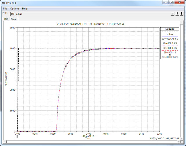
First of all, this issue only comes up for a very small range of data sets in which there are extremely tight constrictions and expansions, and the velocity changes are very extreme (i.e. going from a very low velocity to a very high velocity through the constriction, then back to a low velocity through the expansion).   This is not an issue of high velocity (HEC-RAS can handle high velocity data sets just fine).  Here is an example data set for a river system that is completely straight (i.e. has not contractions/expansions or curves).  The data set is a rectangular channel (200 ft wide) on a constant slope (0.001) that is 10,000 ft long.  The inflow hydrograph goes from 0.0 to 4000 cfs in 10 seconds (like an instantaneous dam or levee breach), then remains constant at 4000 cfs.  The grid size used 40 X 40 ft. grid cells.  So there are 5 cells across the channel.  The maximum velocities vary from a high of around 8 ft/s at the upstream end to around 4.5 ft/s at the downstream end.  Give the 40 ft cell size, and the max velocity of around 8.0 ft/s, a 5 second time step would result in a Courant number of around 1.0 at the upstream end during the max velocity.  All other locations and time will have courant numbers less than 1.0.  I ran this data set with the following time steps: 5, 2, 1, 0.5, 0.2 seconds.  The 0.2 second time step would results in maximum Courant numbers of 0.05 at the upstream end, and even lower everywhere else, as well as when the flood wave is at lower velocities.  The plot below shows the inflow hydrograph and all of the downstream hydrographs for the runs with different time steps.  As you can see, the downstream hydrographs are exactly the same.  This shows that the problem is not an issue of rapidly changing velocity with respect to time, or even distance, if the special velocity changes are not highly curved (as would be the case in severe contractions/expansions, or around sharp bends).


The issue arises for data sets that have extremely high changes in velocity over short distances, and when the path of the velocity is highly nonlinear with respect to space (velocity path is curving over short distances).  However, even in these types of conditions, if the user picks a reasonable time step for these zones, the HEC-RAS model will produce good consistent results.  This is exactly what the EA Test Case 5 shows.  This test case has several very tight constrictions/expansions.  It is also very steep upstream and then becomes very flat downstream.  The velocities in this model are extremely high, in some of the contractions the velocities are between 5 to 6 m/s (16 to 20 ft/s).  Additionally, the models all start out with the downstream area completely dry, then a hydrograph is introduced that goes from zero flow to the peak flow in 5 minutes.  As shown above, if the user picks a reasonable time step with HEC-RAS it can compute a solution that is similar to all of the other listed models in this test case, and is very close to the same results as TUFLOW, Mike21, ISIS 2D, and SOBEK 2D.

The reason HEC-RAS shows variation in the results, when selecting small time steps (far away from a Courant number of 1.0), is due to how we are calculating the convective acceleration terms in the momentum equation.  The current implementation of the 2D “Full Momentum” equations in HEC-RAS 5.0 Beta, uses an Eulerian-Lagrangian formulation (ELM). This is a non-conservative form of the momentum equation which is efficient and accurate for a very wide range of flow conditions.  However, when the convective acceleration terms in the momentum equation are dominant (rapid changes in velocity over short distances), this formulation is accurate within a more limited range of Courant values.
 
When the convective acceleration terms in the equations are dominant, the numerical approximations made in the convective acceleration terms become important. In HEC-RAS 2D the convective acceleration terms are discretized using a Lagrangian formulation which has two steps: a numerical integration on the velocity field, followed by an interpolation process.

If the time-step is too large, the numerical derivatives in the solver will not be appropriate to capture the non-linear behavior of the fluid, driven by high acceleration terms. If the time-step is too small, repeated interpolation to derive the convective acceleration will havea diffusive effect in the velocity field, similar to the smoothing effect of a moving average curve.

This means the user’s need to pay more attention when selecting a time step for the Full Momentum solution for extremely rapidly varying floods that have rapid changes in velocity in space.  Users need to pick a time step that results in a Courant number around 1.0 for the high velocity zones of the simulation.  Picking a time step that is too large (resulting in Courant numbers that are too high, i.e. > 2.0) may result in computational instabilities.  Additionally, for these extremely rapidly varying flow conditions, picking a time step that is way too small (resulting in Courant numbers that are less than 0.1), may result in some numerical diffusion of the computed velocity for certain types of conditions (as described above).

The HEC-RAS Diffusion Wave method does not use the ELM approach in solving the equations.  Therefore this method is not as sensitive to time steps that are too small, and it will ultimately converge on an answer that does not change as you reduce the time step.
Users should always test the consistency of their computational mesh and selected time step.  The consistency principle requires a reduction of both the space (grid) and time steps in order to guarantee convergence of a solution. If the grid is refined and the time-step is reduced simultaneously, the method will achieve convergence.  The user should always test different cell sizes (ΔX) for the computational mesh, and also different computational time steps (ΔT) for each computational mesh.  This will allow the user to see and understand how the cell size and computational time step will affect the results of your model.  The selection of ΔX and ΔT is a balance between achieving good numerical accuracy while minimizing computational time.

Note: people using the current Beta version of HEC-RAS 5.0 will have no trouble getting good results for any data set if they pick a time step based on the guidance provided in the HEC-RAS 2D user’s manual.  So, as far as I am concerned, this is not even an issue for the current Beta release.   However, HEC is currently working on improving this portion of the full shallow water equation formulation, such that user’s will be able to use very small time steps without the results changing significantly.

8.  I read Bill Syme’s contribution to this forum.  First off I would like to say “Thank you” to Bill for being professional and discussing modeling issues in an appropriate professional manner.  I agree with almost all of Bill’s discussion, as I feel that the modeler is the most important thing in producing a good hydraulic model, not the software.  However, I do have a few concerns with Bill’s discussion, as it might imply that HEC-RAS is performing computations in a less robust way than it actually is.  I do not think that Bill Syme was singling HEC-RAS out on these issues, but I do think many people reading his response may think that these comments applied to HEC-RAS.  So I want to set the record straight on a few of his discussion points, as it would pertain to HEC-RAS.  Bill’s comment under Number 2 of his document, does not mention HEC-RAS directly, but it talks about models that solve the 1D shallow water equations on a 2D grid.  HEC-RAS is not doing that!!! HEC-RAS is solving the full 2D Shallow Water Equations with the inclusions of turbulence modeling (Eddie viscosity) and the Coriolis affects.  Point 4 of Bills document talks about 1stand 2nd order accuracy.  As I mentioned previously, in general we are 2nd order accurate in space and time, unless Theta is set to 1.0, then it is first order accurate in time.  Comment 5 also implies that HEC-RAS is 1st order accurate, which is not correct.

9.  There was a comment in the forum that stated that “HEC-RAS was the least accurate and the slowest”.  I think this is an extremely unfair comment. 

First off, we have made significant speed improvements with each Beta version of HEC-RAS.  So it would depend on which version of HEC-RAS 5.0 2D was used.  Second, the HEC-RAS 2D scheme makes use of multiple CPU cores, so the more cores you have, in general the faster it will run.  So what machine was this run on?  How many Cores did it have?  What was the CPU speeds. 

There are other models using GPU solutions.  Models that use GPU solutions are explicit solvers and require time steps that equate to Courant numbers less than 1.0 for all of space and time during the simulation.  However, GPU’s often have 256 or 512 GPU cores on the graphics card.  For large models (100,000 cells and larger) this can produce much faster run times than models like HEC-RAS that are parallelized based on multiple CPU’s.  A GPU formulation will run faster for models with large numbers of cells, but will tend to require a much finer resolution in time and space.  A fair comparison of HEC-RAS 2D against a GPU code would have RAS running with a courser grid that effectively utilizes subgrid bathymetry, and produce the same results.  Under those circumstances HEC-RAS-RAS 2D may provide accurate results with significantly improved run times.

HEC is in the process of working on a GPU version of RAS 2D, but we are just getting started, so it will be sometime before we have a version that can be run on a GPU.

As to the comment about being “Least Accurate”.   This is based on only running the Environmental Agency Test cases, and only about one of the test case, at a single location within that test case (Test case 5, location 5).  As I stated previously, I have run 7 of the 8 test cases and have obtained just as good as results as any of the models applied to those test cases.  This is another example, of the fact that the modeler is more important than the software product.  If a person knows the software really well, which means knowing its strengths and its limitations, they can produce good results for almost any test case.  Unless the model does not have a required capability to perform that test case.  I will be publishing the official HEC results for the Environmental Agency Test cases shortly after the final release of HEC-RAS 5.0.  I want to wait until the final release so the results show exactly what the user would get if they run RAS 5.0 with the data sets in question.

10.  There was also a comment that “TUFLOW was the most efficient from a project perspective (14 times faster than HEC-RAS)”.  This is also an unfair comment.  Project efficiency is in general not about which model runs faster (unless model run times are exorbitant).  Efficiency is about the experience of the modeler using that specific software product, their knowledge of the river system being modelled, their ability to develop a model that accurately reflects the river/floodplain and the events being modelled, and their ability to understand the model results.  In general, HEC-RAS is very easy to use and efficient.  Developing a 2D model is even easier now with the tools we have added to develop a computational mesh that reflects the unique aspects of the river and floodplain, as well as all of the barriers to flow movement. 

What version of HEC-RAS was used for this time comparison?  How many CPU cores did it have? Which version of TUFLOW were you comparing it against?  Did you run it on the same machines?  Were you using the GPU version of TUFLOW, which would have the benefit of possible 512 GPU cores?  Even if you used the exact same machine, and TUFLOW classic, you failed to realize the benefit of HEC-RAS’s ability to utilize the subgrid terrain data in developing the hydraulic property tables of the cells and the faces, as stated previously.  This means that HEC-RAS will allow users to use far fewer cells than the other models, and still produce similar results.  So if you use HEC-RAS, and realize that it has this capability, you will be able to get similar results with much faster run times.  This was the whole purpose of HEC adding this capability into our 2D software.  By ignoring this significant capability within HEC-RAS, you are not really making a fare comparison of run times.  This was not done for this comparison, but I have done this on many data sets and have shown that HEC-RAS can do this with great success.

Additionally, since HEC-RAS can use unstructured grid cells, users can easily align cells along main channel banks (at the high ground that separates channel from overbank flow); along levees; major roads; and other barriers to flow.  This allows for larger cells, while still accurately defining the critical elevations of these flow barriers with the cell faces.  The other models will have to use much smaller cell sizes to pick up the details of these features.  So how can one ensure that the main channel flow carrying capacity is being accurately respected?  The HEC-RAS subgrid terrain approach, unstructured grids, and breakline tools make it easy for user’s to do this within the full 2D domain.

11.  There was a comment that stated: “The intent of the benchmarking testing was to compare each model against recorded data to determine their accuracy using identical inputs (i.e. Cell size, cell topography, etc…)” This statement is not correct.  First off, none of the EA data sets have observed data to compare against, except Test Case 6A, which is an instantaneous dambreak test from a flume experiment.  However, the observed data from this test case is very noisy (jumps around a lot), and none of the models were able to produce very accurate results compared to this observed data.  Some models did better than others of course.

Second, here is a direct quote from page iv of the EA 2013 Benchmarking Test Results document:

               “The overall objectives of this research are to provide:
            1.  an evidence base to ensure that 2D flood inundation modelling packages used for flood risk management by the Environment Agency and its consultants are capable of adequately predicting the variables on which flood risk management decisions are based
            2.  a data set against which such packages can be evaluated by their developers”

            Please take special note to Item 2 above.  It was always the original intent of the Environmental Agency to see if a model could actually perform these tests, but based on their most appropriate application of the test problem and the software being used.  As you know, it is very easy for someone who is not truly an expert in a particular piece of software, to unintentionally misapply that piece of software.  This is why the Environmental Agency wants the model developers to apply these test data sets and report the results in a public form.  This does not mean that user’s should not also run these tests, or any other tests that they feel are important in their model selection.  However, if you are not getting the same results as HEC on these specific test cases, then you may not be using HEC-RAS to its fullest extent/capability.

12.  There was a comment that stated: “a triangular mesh is better suited to describe a 2D flow behavior because you can compute 3 different flow directions for each cell instead of just 2 as happens for quadrangular meshes”.  This is not correct.  As far as I know, flow can cross a cell face at any angle for all of these models in this discussion.  This is definitely true for HEC-RAS.  HEC-RAS can use triangles, squares, rectangles, and cells up to eight sides.  So the mesh can be structured (square grids) or completely unstructured with cells of varying shapes and sizes.  Water can cross the face of any cell at any angle (360 degrees).  I have performed many test experiments where I have aligned the grid in the direction of flow, then took the same model and purposefully aligned all faces at 30, 45, and 60 degrees to the direction of flow.  HEC-RAS produces almost the exact same results, with very little variation.  This is something we spent a lot of time on to get it right.  Without this being true, no unstructured mesh software would ever be able to solve flow movement for any real world channel and floodplain.


Some final thoughts:

1.       All of these 2D models produce different results for all of the 8 EA test cases.  Some are closer together than others, but none are the same.  Yet they are all solving the 2D shallow water questions (except of few of the models, which are clearly pointed out in the study). 
 
2.      There are many things that will cause different results to occur with these different models, such as:
a.      Mesh size, shape
b.      Time step
c.       How each model depicts the actual terrain within their mesh (Cells and faces).  As I mentioned above.
d.      Friction modeling
e.      Temporal and convective acceleration modeling
f.        Turbulence modeling
g.      Etc..

3.      It is absolutely true that the modeler is more important than the software selected.  A person who is a good hydraulic modeler needs to have the following qualities:

a.      A good understanding of river hydraulics both in theory and practice (real world water movement).
b.      A good understanding of hydrology, as all of these hydraulic models require accurate inflow boundary conditions to have any chance of predicting a good result.
c.       A reasonable understanding of numerical analysis as it applies to solving equations such as the shallow water equations.  This means understanding how grid resolution and time step selection will influence model results.  As well as a reasonable understanding of how the other terms in the momentum equation are being computed, and there significance to your specific study.
d.      A good understanding of the system they are modeling and how it will react to the events they are modelling.
e.      Knowledge of special hydraulic features, such as: levees, bridges, culverts, dams, weirs, spillways, pump stations, etc… and how to best model these features with the software you are using.


4.        None of the test case discussed in this forum have any observed data.  So no one can truly say which model is producing better results.  Many things will affect the results that the models produce, and there are different plusses and minuses of each of the software packages.

The Advanced Hydrologic Prediction Service for Chehalis Washington

$
0
0
A great example of where flood inundation maps and accessible flood warning systems can help a community prepare for floods.


Contact:               Brent Bower                                                                      FOR IMMEDIATE RELEASE 
206-526-6095 x228                                                           December 15, 2015
                               
Flood Inundation Maps to Enhance Flood Forecasts for the Chehalis River

People living along the Chehalis River have a new tool from the National Weather Service to help them understand their risk during floods. A large section of the river is now depicted on flood maps that show people where the water will flow and what it will look like in their community when the river crests beyond its banks. The new flood inundation maps will also help local officials reduce flood impacts to communities by giving them more advanced information for planning.


The Advanced Hydrologic Prediction Service (AHPS) flood inundation map project for the Chehalis River demonstrates the National Weather Service’s commitment to identify specific flood impacts and help communities become more weather ready. When the National Weather Service issues river forecasts, residents and businesses will be able to use the maps of water levels for different stages to see what their flood threat is, and take action to protect themselves and their property.

The Centralia/Chehalis area is only the second western U.S. location after Boise to get the maps, which are available in 130 other locations with more being added all the time. The maps were produced in partnership with the Chehalis River Basin Flood Authority and their contractor, WEST Consultants, with the assistance of the local stakeholders – City of Centralia; City of Chehalis; Lewis County; Washington State Departments of Transportation, Ecology, and Emergency Management;  FEMA; and the U. S. Army Corps. of Engineers, Seattle District.

The flood maps are available in the AHPS webpage.

NOAA's National Weather Service is the primary source of weather data, forecasts and warnings for the United States and its territories. NOAA’s National Weather Service operates the most advanced weather and flood warning and forecast system in the world, helping to protect lives and property and enhance the national economy. Working with partners, NOAA’s National Weather Service is building a Weather-Ready Nation to support community resilience in the face of increasing vulnerability to extreme weather. Visit us online at weather.gov and on Facebook.


On the Web:
NOAA’s National Weather Service: http://www.weather.gov

NOAA’s National Weather Service Seattle: http://www.wrh.noaa.gov/sew/

HEC-RAS 2D Training in Australia!

$
0
0
Alright Aussies!  Time to step up.  Who wants some HEC-RAS 2D Modelling training?   This will be a fantastic opportunity to learn how to set up and run 2D and 1D/2D HEC-RAS models.  Mr. Krey Price and I will be hosting this course in two locations in Australia this year:  Brisbane March 2-4 and Melbourne March 7-9. Please go here for more details and to register your interest.


Following the success of his 2015 HEC-RAS 5.0 course held in Italy, former HEC-RAS Development Team Member Chris Goodell will be travelling to Australia in March 2016 to conduct two intensive 3-day courses focused on 2D model development in HEC-RAS.

Following are the dates for the courses:
* Brisbane 2-4 March 2016
* Melbourne 7-9 March 2016

The courses will be held in CBD conference/training facilities. Venues will be finalised in the next few weeks based on response, with additional cities added subject to demand. Please register your interest at http://www.surfacewater.biz/register-your-interest/and fill out the survey, so we can plan appropriately for the class size.


Chris is the Director of Applied Research for WEST Consultants, Inc. and is the author of the popular blog "The RAS Solution".  He has numerous publications about advanced capabilities within HEC-RAS, including his book "Breaking the HEC-RAS Code," which presents the use of the HECRASController in customising HEC-RAS for Monte Carlo simulations and other specialised model runs.

Chris will be assisted by Krey Price, a hydraulic modeller who recently supervised a 6-month benchmarking study on over 200 model runs comparing the beta version of HEC-RAS 5.0 with TUFLOW. Krey has 15 years of consulting experience for the U.S. Army Corps of Engineers, including dam breach, levee design, and sediment transport modeling and seven years of hydraulic modelling experience for Australian industries and public agencies.

In addition to presenting 2D functionality, the course will also include an introduction into sediment transport capabilities within HEC-RAS as well as presenting the results of several recent benchmarking studies comparing HEC-RAS 5.0 to other industry-standard models, including TUFLOW and MIKE. Additional details on the course contents are included on the website http://www.surfacewater.biz/course-outline-and-contents/.

Contact details for further questions can be found at www.surfacewater.biz.

Is it normal with a 2D full momentum model to run without any WSEL errors? Or should I expect a few?

$
0
0
Written by Christopher Goodell, P.E., D.WRE  |  WEST Consultants 
Copyright © The RAS Solution 2016.  All rights reserved.   

You can have a 2D full momentum model without errors if:

  • Your cell size and computation interval is appropriate
  • Everything is moving very slowly
  • Stages are high
  • Slopes are shallow
  • N values are high
  • Discharge doesn’t change too suddenly
  • It’s a 2D only model (i.e. no connections to 1D)
  • You are a skilled HEC-RAS modeler
  • A combination of any or all of these (and some other factors I’m not thinking of), sure, you can have no errors. 
Is it normal?  I certainly wouldn’t call it abnormal.  Actually, you’d be surprised at how well the 2D solution works compared with the 1D solution.  I’ve found I get a lot less errors and instabilities in 2D areas than I do with 1D reaches.  Most of the time, my big errors happen at and around 1D/2D connections.

If you are lucky to get a simulation with no errors, double check your solution-make sure it looks reasonable.  Your instincts are correct and you should question the results.  But if everything looks good and reasonable, chalk it up to your skill and claim your bragging rights! 

Post-Processing: Creating Inundation Maps with very Large Terrain

$
0
0
Written by Mikell Warms  |  WEST Consultants 
Copyright © The RAS Solution 2016.  All rights reserved.   

We often have to deal with very large models covering hundreds of river miles.  The terrain data associated with these models can be equally massive, which can cause memory/processor issues when trying to delineate inundation maps.

This post is not concerned with pre-processing our model geometry. Instead, we have a completed model with results we are happy with, and now we want to make inundation shapefiles. This is often necessary when completing dam breach analyses/flood analyses/etc. 

There are typically two ways in which flood inundation shapefiles are created: (1) using HEC-GeoRAS and (2) RAS Mapper. Both methods can face uphill battles when terrain data begin to exceed 20-30 gigabytes, depending on performance characteristics of your computer. Below are some typical errors you may see when trying to create inundation shapefiles with RAS Mapper on very large terrain.


Figure 1: RAS Mapper Memory Error Messages

There IS a way to get around this using RAS Mapper. The first thing you’ll need to do is
Clip your terrain into smaller, more manageable pieces using your favorite GIS software. In this example I’ve used ArcGIS. In ArcMap, it is easy to clip terrain using a clipping shapefile and the Clip tool under Data Management > Raster > Raster Processing. For this example, I’ve clipped my terrain into 12 terrain pieces.


Figure 2: Clipped Terrain over Columbia and Deschutes Rivers downstream of John Day Dam

You may find (as I did), that your initial terrain splitting will not be quite enough, so you may have to complete this step again.

Next: Use RASMapper to convert ALL of your DEM pieces into terrain usable by RAS. Make sure all of your DEM pieces are in the project’s projected coordinate system.

If converting ESRI grids to RAS terrain, any of the many files that make up the ESRI Grid  can be chosen by the terrain creator window:


Figure 3: ESRI Grid file format


Figure 4: Clipped ESRI Grids converted to RAS terrain using RAS Mapper (look at all of those terrain files!)


Figure 5: Creating RAS terrain layers in RAS Mapper

The next steps will have to be repeated for as many terrain pieces as you have. Start by associating the first terrain piece to the results of the plan you wish to map (Right click on Results in the Layer Manager in RAS Mapper > Manage Geometry Associations):


Figure 6: Associating terrain layers with geometry and results in RAS Mapper


Make sure that RASMapper has mapped the depth grid (or any other result) over that terrain piece before proceeding. You may have to click inside the RASMapper window and pan around to get the map to update.


Figure 7: Note that the depth grid is plotted over the correct terrain piece.


Next, right click on Resultsin the Layer Manager in RAS Mapper, and select Manage results maps.


Figure 8: Manage Results Map Menu in RAS Mapper

If you have more than one plan’s results in the menu, make sure to choose the plan or plans that you are interested in mapping. Select Add New Map from the menu. Choose Depth or Inundation Boundary as your Map Type, a Maximum Profile from the Unsteady Profile Menu, and Polygon Boundary should be set to 0. You can name the Layer anything you would like, although naming it something similar to your terrain piece would be helpful. Click Add Map.


Figure 9: Results Map Parameters Menu in RAS Mapper

  
We’re not finished yet, RAS Mapper still has to Compute the map properties and create the shapefile. In RAS Mapper, Right Click on the added map and choose “Compute/Update Stored Map”.


Figure 10: We have to tell RAS Mapper to compute the added maps/inundation shapefiles

This is where you will figure out whether or not your terrain pieces are small enough. If the terrain pieces are still too large, you may get one of the error messages shown above. If you succeed in creating your inundation shapefile, repeat this process until you have created shapefiles for all of your terrain pieces.

Once all of the inundation shapefiles have been completed, return to your favorite GIS software and add the inundation polygons to your map.


Figure 11: Unmerged inundation shapefiles.

Note: In the above figure, there are some split channels that are not included in the inundation. This may be caused by errors in the model or the terrain extent may not be large enough for the inundation. Prior to completing the next step, ensure that all of your individual pieces are correct. For this analysis, we were not concerned with this section of the inundation so it was not addressed.  
Next, merge the polygons to create one large polygon. In ArcGIS, the Merge tool under Data Management > General in the Toolbox can be used to easily merge the shapefiles.


Figure 12: Merging Inundation Shapefile Pieces

You have now created an inundation shapefile over a very large area and can proceed to make detailed inundation maps for your project.


Figure 13: Finished Product

HEC-RAS 2D Training in Melbourne Australia is Official - April 5-7, 2016

$
0
0
The 2D HEC-RAS class is a GO!  Who wants some HEC-RAS 2D Modelling training?   This will be a fantastic opportunity to learn how to set up and run 2D and 1D/2D HEC-RAS models.  Mr. Krey Price and I will be hosting this course in Melbourne, Australia on April 5, 6, and 7th. Please go here for more details and to register for the class.  There will be some additional courses throughout Australia later, but I will only be participating in the Melbourne class on April 5, 6, and 7th. 


Following the success of his 2015 HEC-RAS 5.0 course held in Italy, former HEC-RAS Development Team Member Chris Goodell will be travelling to Australia in April 2016 to conduct two intensive 3-day courses focused on 2D model development in HEC-RAS. 


This course will take place in  Melbourne,  5-7 April, 2016.

The course will be held in CBD conference/training facilities in downtown Melbourne. Please register for the class at http://www.surfacewater.biz/register/.

HEC-RAS 5.0 Official Release is Available!!!

$
0
0
The wait is over!  Finally the official release of HEC-RAS Version 5.0 is here.  You can download it from the HEC website at http://www.hec.usace.army.mil/software/hec-ras/

This new version also comes with updated manuals (User's Manual, Hydraulic Reference Manual, and Applications Guide), as well as a new 2D Modeling Manual.

Enjoy and good luck!!!

HEC-RAS 2D Training in Portland Oregon

$
0
0

I'll be teaching our very popular 2D HEC-RAS course in my home town of Portland Oregon, just in time to feature the official release of HEC-RAS 5.0.  

If you live in the area, or you've always wanted to figure out why everyone is talking about Portland (and HEC-RAS 5.0!), read on for more information and to register.  

This course is being hosted by River Restoration Northwest.  Please contact them for course registration questions.

River Restoration Northwest Presents
 a course in HEC-RAS 2D Modeling
JOIN US in Portland, Oregon!

April 11-13, 2016
8:00 AM - 5:00 PM Every Day
Fee: $700
Registration is now open. 
Location: Cheatham Hall at the World Forestry Center in Portland
Instructor: Chris Goodell, WEST Consultants
NOTE:  Course fees are non-refundable except in the event that minimum course registration numbers are not met.  
The Army Corps of Engineers Hydrologic Engineering Center’s River Analysis System (HEC-RAS) has been updated to include two dimensional modeling capabilities. This intensive 3-day workshop will introduce the experienced HEC-RAS user to these new 2-D capabilities.
Through attending this workshop, participants will:
  • Learn how to use the U.S. Army Corps of Engineers HEC-RAS (River Analysis System) computer program to model two-dimensional unsteady flow hydraulics.
  • Get an overview of two-dimensional flow theory and the differences between one-dimensional and two-dimensional modeling.
  • Gain hands-on HEC-RAS experience by participating in practical computer workshops.
  • Understand how to develop a stable and calibrated two-dimensional flow model.
  • Obtain valuable insights in methods for minimizing computation errors and instabilities for two-dimensional unsteady hydraulic models.
  • Learn from real world projects and applications.
Instructor:
Christopher R. Goodell, P.E., D.WRE, is a senior hydraulic engineer with WEST Consultants with over 20 years of experience in computational hydraulics, river hydraulics and hydraulic design. He spent two years at the Hydrologic Engineering Center (HEC) actively working on the development of HEC-RAS. In addition, Mr. Goodell is a contributing author to the HEC-RAS manuals and has applied HEC-RAS to a wide range of complex problems, including dam breaks, bridge and culvert hydraulics, spillway and outlet works design, stable channel design, and floodplain mapping. Mr. Goodell earned his B.S. degree in civil engineering at Oregon State University and his M.E. degree in hydraulic engineering from the International Institute for Hydraulic Engineering (IHE) in Delft, The Netherlands. Mr. Goodell has taught HEC-RAS courses and provided technical support for HEC-RAS since 2000.
CLASSROOM LOCATION:
Your class will be held in the WORLD FORESTRY CENTER at 4033 SW Canyon Road, Portland, OR, 97221. The office phone number is 503-228-1367. Our class will be held in Cheatham Hall that is located to the south of the Discovery Museum and Plaza.
LOC
DIRECTIONS:
By Car
Located in Portland's Washington Park, the World Forestry Center is just five minutes from downtown Portland. For detailed driving directions please visit the World Forestry Center’s website at:http://www.worldforestrycenter.org/organization/visitus.php
Portland Parks and Recreation owns and manages parking spaces in Washington Park. They have implemented pay-by-space meters for all patrons who use the park, including those attending events.
Fees: $1.60/hour (9:30AM – 9:30PM) * $4.00/day October-March * $6.40/day April - September
Please visit this link for more detail on the parking meters: http://washingtonparkpdx.org/parking/
TriMet
MAX (Metropolitan Area Express) runs through downtown from the suburbs to the west and east, from the airport, and from the Expo Center. Washington Park has its own MAX stop, which lets you off right at the World Forestry Center’s front door. Check out TriMet’s web site at www.trimet.org for route maps, fares, connections and schedules.
LODGING:
If you need a place to stay, many of the downtown Portland hotels are within easy walking distance to the MAX light rail that provides easy access to Washington Park as described above. The Portland Oregon Visitors Association (POVA) can advise you on Portland-area hotels and motels and book your reservation over the phone. Call toll-free 1-87-PORTLAND (1-877-678-5263) or visit their web site,www.travelportland.com.

Post-Processing with RAS Mapper: Exporting a Large Number of Results Maps

$
0
0
Written by Shaina Sabatine  |  Watershed Science & Engineering, Seattle, WA
Copyright © The RAS Solution 2016.  All rights reserved.

The new and improved RAS Mapper interface in HEC-RAS 5.0 makes managing and exporting model results like an inundation extents shapefile or a depth grid for use outside of HEC-RAS/RAS Mapper easy.  The process (which is described in detail in Chapter 5 of the HEC-RAS 5.0 2D Modeling User’s Manual) requires the user to add desired results maps one by one using the ‘Add New Map’ button in the ‘Manage Results Maps’ window shown in Figure 1 below.

Figure 1: Manage Results Maps window for the results of a completed simulation.  Two results layers have been exported: an inundation boundary shapefile and a depth grid.

Imagine you have a large number of outputs from a simulation that need to be exported.  Because only one new results map can be added to the list in the ‘Manage Results Maps’ window at a time using the ‘Add New Map’ button, the process can become tedious.  One way to make the process
faster is to directly edit the file that is created in your project directory with the extension “.rasmap”.  This is a text file in XML format that RAS Mapper uses to identify the Geometries, Results, Map Layers, and Terrains that it will load into the interface along with some other settings (see Figure 2).

Figure 2: XML document tree showing the elements in a “.rasmap” file.

Each executed plan in a RAS project is listed as a <Layer> sub-element under the <Results> element, and each results layer that RAS Mapper will display is described in another <Layer> sub-element underneath that (see Figure 3).  Note: the saved results of a HEC-RAS 5.0 simulation are stored in the file with the extension “.p##.hdf” where ## denotes the plan number. The “.rasmap” file stores information about outputs from the “.p##.hdf” file that will be displayed in the RAS Mapper interface.


Figure 3: XML document tree for the “.rasmap” file associated with the results in the window shown in Figure 1.  The tree has been expanded to show plan <Layer> sub-elements and result <Layer> sub-elements which are under the <Results> element.

Figure 3 shows that 6 results layers will be loaded into RAS Mapper for the plan named “RampFlows2DArea” including an inundation polygon for January 02 at 00:00:00 and a depth grid for January 02 at 00:00:00.  Say you would like to export inundation polygons and depth grids for multiple more profiles in this plan.  Because the “.rasmap” file is simply a text file, it can be opened in a text editor and manipulated.  In this example, one inundation polygon and one depth grid have already been created for the “RampFlows2DArea” plan.  Rather than adding each additional desired results map layer using the ‘Add New Map’ button in the RAS Mapper interface (Figure 1), the “.rasmap” file can be directly edited.  Additional desired results maps can be added by copying the associated block(s) of text, pasting a block in the correct location for each desired results map, and editing as needed.  At a minimum, both the name of the layer and the date/time of the profile being exported will need to be edited (see Figures 3 and 4).  **IMPORTANT- do not have HEC-RAS open while editing the “.rasmap” file.** 

Figure 4: Example of the edited “.rasmap” file.  Blocks of text were inserted for profiles for January 03 through January 07 at time 00:00:00.  The red boxes highlight where edits were made.

Figure 4 shows a portion of what was edited in the “.rasmap” file.  The red boxes in Figure 4 highlight where edits were made.  In this example, it was desired to have an inundation boundary and a depth grid exported for every simulated day at time 00:00:00.    After editing the “.rasmap” file, save it and open your HEC-RAS project and then RAS Mapper.  The results maps will be listed under their plan name under Results in RAS Mapper as shown in Figure 5.

Figure 5: Inundation boundary and depth grid results maps loaded into RAS Mapper after editing the “.rasmap” file.

Inundation boundaries and depth grid results maps have been loaded into RAS Mapper for every day from January 02 through January 20 at time 00:00:00.  Note that a red asterisk means a map has not been created or exported yet.  To create/export maps, select all of the maps and click ‘Compute/Update Stored Maps’ in the ‘Manage Results Maps’ window as shown in Figure 6.

Figure 6: Selecting and creating/exporting the results maps.

Now, all you have to do is wait.  Exporting this many layers could take a while.  Note: This model run was set up so that all the profiles that needed to be exported were at time 00:00:00.  This is why the time stamp was not edited in the “.rasmap” file.


Experiences with the new HEC-RAS v5 for 2D river flood simulation

$
0
0
A nice replication of the Mamore Flood of 2014 in Bolivia using HEC-RAS Version 5 courtesy of Vladimir Moya.


Viewing all 200 articles
Browse latest View live